Error correction
Reading time: 16 minutes
Contents
- What is error correction?
- Longer computations need more qubits
- What is the current state-of-the-art?
- Conclusion
- See also
Around 2024, we’re seeing a major shift in the road maps of quantum computer manufacturers. Several companies no longer put their bare qubits in the spotlight, but instead focus on logical qubits. Error correction seems to be an essential component of large-scale quantum computing, adding yet another facet in which these devices differ from their classical counterparts. Although this is a relatively advanced topic, we find it so important that it deserves a dedicated chapter in this book.
As with many aspects of quantum computing, error correction can be rather confusing. A statement that we often hear is the following (which is incorrect!)
‘Logical qubits (or error-corrected qubits) are resilient to errors that occur during a computation. Once we have logical qubits, we can increase the length of our computations indefinitely. ‘
What’s the problem here? Well, not every logical qubit is created equally. In the near future, we expect to see logical qubits that are perhaps 2x more accurate than today’s bare hardware qubits, and later 10x, and in the future perhaps 1000x. Error correction is a trick to reduce the probability of errors, but it will not eliminate errors completely. In the following decade, we expect gradual improvements, hopefully down to error rates of 10-10 and below.
What is error correction?
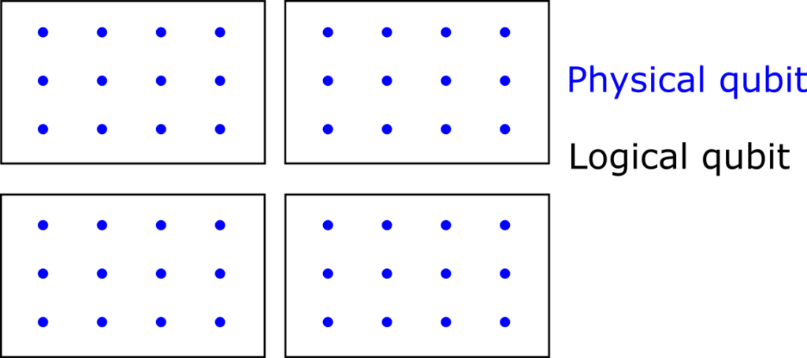
In quantum error correction, we combine some number (think of hundreds or thousands) of ‘physical’ hardware qubits into a virtual ‘logical’ qubit. The logical qubits are the information carriers used in an algorithm or application. Error correction methods can detect whenever tiny errors occur in the logical qubit, which can then be ‘repaired’ with straightforward operations. Under the assumption that the probability of hardware errors is sufficiently low (below a certain error threshold), the overall accuracy improves exponentially as we employ more physical qubits to make a logical qubit. Hence, we obtain a very favourable trade-off between the number of usable qubits and the accuracy of the qubits.
Doesn’t measuring a quantum state destroy the information in the qubits?
Indeed, if we naively measure all the physical qubits, we destroy potentially valuable information encoded in the qubits. However, quantum error correction uses an ingenious way to measure only whether or not an error occurred. It learns nothing about the actual information content of the qubit. It turns out that this way, the data stored in the logical qubit is not affected.
Why are errors so much of a problem? How do errors screw up our computations?
In short, even tiny errors are a problem because we want to perform an astonishing number of quantum operations successively — think of billions or trillions of them.
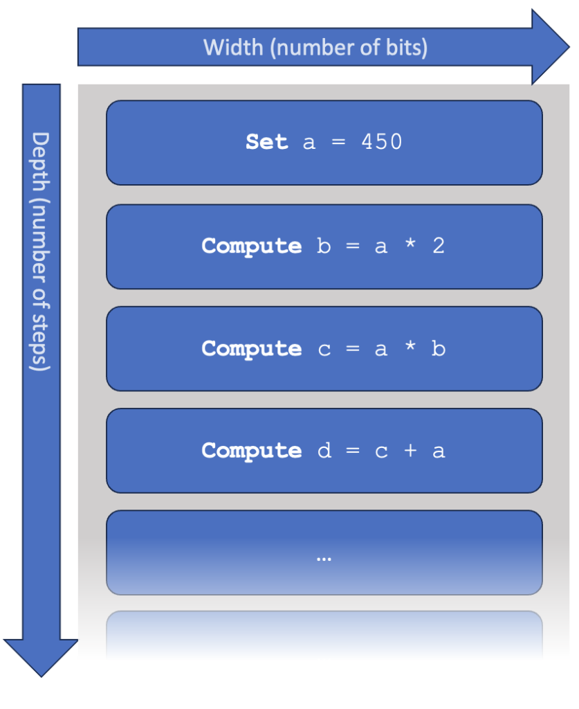
Let’s make this more concrete. A computer program is essentially a sequence of ‘steps’, each of which a computer knows how to perform. We say that a program or algorithm has a width, which is the number of qubits it requires. It also has a depth, which is the number of consecutive steps that need to be performed. You may interpret one step in early hardware as a single quantum gate (although, in practice, gates may be performed in parallel, making the impact of errors slightly more complicated).
The concept of ‘width’ is pretty straightforward: if the computer doesn’t have enough memory, it cannot run the program. Dealing with ‘depth’ is harder. To run a program of 109 steps, we need to limit errors to roughly the inverse, say, a probability of 10-9 per step. If the error is larger, it becomes extremely unlikely that the quantum computer will produce the correct outcome. These are not hard numbers: a computer with 10-10 error would be a significant improvement (resulting in much fewer mistakes), and a computer with 10-8 error might be pushed to also find the correct answer after many tries. However, as the imbalance between depth and error grows, the probability of finding a correct outcome is reduced exponentially. We illustrate this in more detail in the box below.
To illustrate, why do we need such small error rates?
Let’s look at a very simple model of a computer, which is not unlike what happens inside a quantum computer or a modern (classical) CPU. As above, the computer is supposed to work through a list of instructions. We can consider various specifications of a computer:
- The available memory, measured in bits (or perhaps megabytes or gigabytes, if you like).
The speed at which the computer operates, measured in steps per second.
The ‘probability of error’, describing the likelihood that one gate introduces some mistake. This is given as a number between 0 and 1 (or a percentage between 0 and 100%). Many sources use the word ‘fidelity’ instead, which can be roughly interpreted as the opposite (fidelity ≈ 1 – probability of error). In this text, we sometimes just say ‘error’ while we mean its probability.
In this simple model, the time taken to complete the computation equals ‘depth’ x ‘speed’. You can make the calculation faster by increasing the speed of the computer or by writing a ‘better’ program that takes fewer steps.
The influence of errors is harder to track. For contemporary computers, we typically don’t worry about hardware mistakes at all, as every step has essentially 100% certainty to output the correct result. However, let’s see what happens when this is not the case.
Assume that each step has a 1% (= 10-2) probability of error. What will the impact be on the final computation? Below, we compute the probability to finish the computation without any errors, for various numbers of computational steps.
| Error probability: 1% | |
|---|---|
| Number of steps | P(success) |
| 1 | ( 0.99 )1 = 99% |
| 100 | ( 0.99 )100 = 37% |
| 1000 | ( 0.99 )1000 = 0.004 % |
| 10,000 | ( 0.99 )10,000 = 10-44 |
In this simple model, we assume that any error is catastrophic. This is quite accurate for most programs. You might argue that there is a miniscule probability that two errors cancel, or that the error has very little effect on the final result, but it turns out that such effects are statistically irrelevant in large computations.
Now, if we improve the hardware to have an error rate of just 0.1% (=10-3), we find the following.
| Error probability: 0.1% | |
|---|---|
| Number of steps | P(success) |
| 1 | ( 0.999 )1 = 99.9% |
| 100 | ( 0.999 )10 = 90% |
| 1000 | ( 0.999 )1000 = 37% |
| 10,000 | ( 0.999 )10,000 = 0.004 |
A 37% probability of succeeding may sound bad, but for truly high-end computations, we might actually be okay with that. If the program results in a recipe for a brand-new medicine or tells us the perfect design for an aeroplane wing, then surely we don’t mind repeating the computation 10 or 100 times, after which we’re very likely to learn this breakthrough result. On the other hand, if the probability of success is 10-44, then we will never find the right result, even if the computer repeats the program billions of times.
In the table above, we see a pattern: to reasonably perform 102 steps, we require errors of roughly 10-2 or better. To perform 103 steps, we need roughly a 10-3 probability of error. These are very rough order-of-magnitude estimates, but they lead to a very valuable conclusion when dealing with very large circuits (or very small errors): if you want to execute 10n steps, you’d better make sure that your error probability is not much bigger than 10-n.
This simplified model assumes that an operation either works correctly or fails completely, with nothing in between. In reality, quantum operations act on continuous parameters, and therefore, they have an inherent scalar-value accuracy. For example, a quantum gate with 99% accuracy might change a parameter from A to A+0.49, where it’s supposed to do A+0.5. Luckily, for our discussion, these details don’t matter much. It suffices to see a ‘99% accurate’ quantum gate as simply having a 99% probability of succeeding. We also overlook various other technical details, like operations carried out in parallel, different types of errors, native gate sets, connectivity, and so forth — these make the story much more complicated but will not change our qualitative conclusions.
Why don’t we just make the hardware more stable?
To some degree, we can further reduce errors by creating more accurate hardware. However, quantum objects are so incredibly fragile that even getting down to 10-2 errors requires some of the world’s most astonishing engineering. We definitely hope to see two-qubit gate errors reduced to 10-3 and perhaps even 10-4, but achieving targets of 10-9 seems unlikely with incremental hardware engineering alone. On the other hand, quantum error correction is incredibly effective: the error drops dramatically at the cost of adding a modest number of qubits, which is assumed to be scalable anyway. That’s why experts agree that error correction is the right way forward.
Do we use error correction in classical computers too?
This might be a good moment to appreciate the incredible perfection of classical computer chips. While doing billions of steps per second, running for months in a row, sometimes with hundreds of cores at a time, errors in CPUs practically never occur. I was hoping to find hard numbers on this, but companies like Intel and AMD seem to keep this under stringent non-disclosure agreements. However, some research shows that errors well under 10-20 are easily attained as long as we don’t push processors to their limits (in terms of voltages and clock speeds), sufficiently low that error correction is rarely needed.
Memory (RAM) for high-performance computers still frequently has built-in error correction, and some form of CPU error correction was sometimes used in older mainframes and (even today) in space probes.
Longer computations need more qubits
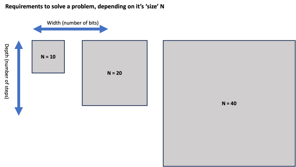
As problems become more complex, they typically require better computer hardware, both in terms of width (number of bits) and depth (number of steps). We could illustrate this below. We define a number ‘N’ that indicates the difficulty or the size of the problem. For example, we might consider the task of ‘factoring a number that can be written down using at most N bits’).
Remember that we’re talking about the requirements to solve a problem, so here, width indicates logical bits. If a computer does not have error correction, then one logical bit is simply the same as one physical bit – or its quantum equivalent.
For ‘perfect’ classical computers, the situation is straightforward: if a problem gets bigger, we need more memory, and we need to wait longer before we obtain the result. For (quantum) computers that make errors, the situation is more complex. With increasing depth, not only do we need to wait longer, but we also need to lower the error probabilities and, hence, need more extensive error correction.
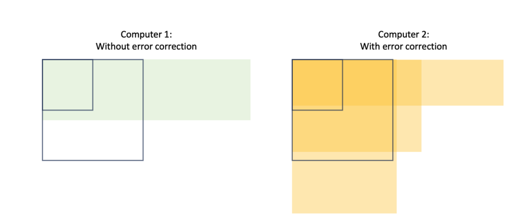
Let’s consider two computers for which we show the width and depth that they can handle (where the available ‘depth’ is assumed to be 1 / ‘probability of error’). On the left is a computer without error correction (hence, it has a small, fixed depth). The other is an error-corrected computer that can trade between depth and width (in certain discrete steps).
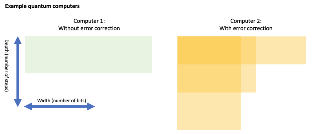
The computer without error correction might have enough memory to solve a problem but often lacks the depth. Even an error-corrected computer might not have a suitable trade-off to solve the hardest problems. Looking at the above example, it seems that both computers can solve the N=10 problem. Here, only the error-corrected computer can solve the N=20 problem, as depicted below. For the N=40 problem, which would be represented by an even larger box, the error-corrected computer might have sufficient depth OR sufficient width, but it doesn’t have both at the same time. Hence, neither computer could solve the N=40 problem.
Towards cracking the N=40 problem, our best bet is to upgrade the error-corrected computer to have more physical qubits. Using error correction, these can be traded to achieve sufficient depth (whilst also reserving just enough logical qubits to run the algorithm).
We have found a paradoxical conclusion here. Larger problems not only require more memory (to store the calculation) but also more depth, which requires more qubits again! To summarise:
‘Harder’ problems -> More depth -> Better error correction -> More physical qubits
Once we reach an era of error correction, scaling the number of physical qubits will still be at the top of our wishlist, as this will be the key enabler of longer computations.
What is the current state-of-the-art?
This section is more technical and can be safely skipped. As of 2024, there have been several demonstrations of error correction (and the slightly less demanding cousin: error detection), but these have all been with limited numbers of qubits and with very limited benefit to depth (if any at all). However, we seem to be at a stage where hardware is sufficiently mature that we can start exploring early error correction.
Below are the three most popular approaches to error correction. Each of them can be considered a ‘family’ of different methods based on similar ideas:
Surface codes
Colour codes
Low-Density Parity Check (LPDC) codes
The surface code (or toric code) has received a lot of scientific attention, as this seems to be on the roadmap of large tech companies like Google and IBM. Their superconducting qubits cannot interact with each other over long distances, and the surface code can deal with this limitation. Many estimates that we use in this book (such as the resources required to break RSA or to simulate FeMoco) are based on this code. It has already been tested experimentally on relatively small systems:
A team from Hefei/Shanghai experiments with a 17-qubit surface code.
Google sees improvements when scaling the surface code from 17 to 49 qubits.
Colour codes are somewhat similar to surface code but typically lack the property that only neighbouring qubits have to interact. This makes them less interesting for superconducting or spin qubits, but they appear to work extremely well for trapped ions and ultracold atoms.
(Scientific presentation) Startup QuEra demonstrates 48 logical qubits using a colour code
LDPC codes are now rapidly gaining attention. They build on a large body of classical knowledge and could have (theoretically) more favourable scaling properties over the surface code.
- French startup Alice & Bob is aiming for a unique combination of ‘cat qubits’ together with LDPC codes, which can theoretically match very elegantly.
Which code will eventually become the standard (if any) is still completely open.
What are the main challenges?
Firstly, we would need just slightly more accurate hardware. We mentioned a certain accuracy threshold earlier: state-of-the-art hardware seems to be close to this threshold but not comfortably over it. Secondly, error correction also requires significant classical computing power, which needs to solve a fairly complex ‘decoding’ problem within extremely small time bounds (within just a few clock cycles of a modern CPU). Classical decoding needs to become more mature, both at the hardware and the software level. It is not unlikely that purpose-built hardware will need to be developed, which for some platforms might be placed inside a cryogenic environment (placing stringent bounds on heat dissipation). Theoretical breakthroughs can still reduce the requirements of classical processing.
Lastly, it turns out that ‘mid-circuit measurements’ are technically challenging. Without intermediate measurements, one might retroactively detect errors, but one cannot repair them. We should also warn that many related terms exist, such as ‘error mitigation’ and ‘error suppression’. They might be useful for incremental fidelity improvements, but they don’t bring an exponential increase in depth like proper error correction does.
Conclusion
The bottom line is that one shouldn’t naively take ‘logical qubits’ as perfect building blocks that will run indefinitely. A logical qubit is no guarantee that a computer has any capabilities; it merely indicates that some kind of error correction is applied (and it doesn’t say anything about how well the correction works). A much more interesting metric is the probability of error in a single step (in jargon: the fidelity of an operation), which gives a reasonable indication of the number of steps that a device can handle!
See also
The Quantum Threat Timeline Report asked several experts what they find the most likely approach to fault-tolerance (section 4.5).
British startup Riverlane builds a hardware chip that ‘decodes’ which error occurred on logical qubits. (Technical report).
Craig Gidney (Google) has a more technical blog post on why adding physical qubits will remain relevant in the following decades.
[Technical!] Some scientific work speaks of ‘early fault-tolerant’ quantum computing, such as:
‘Early Fault-Tolerant Quantum Computing’, discussing how we can squeeze as much as possible out of limited devices.
‘Assessing the Benefits and Risks of Quantum Computers’ takes a similar width x depth approach as we do here, but uses it to assess what applications will be within reach first.